Useful Fundamentals for Path Tracing: Part 4
In a nutshell: Radiometry and photometry are 2 different types of measurements. Photometry is better suited for expressing light intensities in the context of human vision, so its more intuitive for artists. There are a number of different path tracing methods and nowadays use of deep learning and differential rendering are being given more attention in research. For production rendering, unidirectional path tracing with clever sampling strategies is still by far the most popular due to its ease of use for artists.
In this post, we will wrap up by covering some basics on radiometric measurements vs photometric measurements with regards to light, and also run through different potential methods of path tracing.
Radiometry and Photometry
Let’s start with radiometry and photometry. Just incase you aren’t familiar with the differences, radiometry is the science of measuring electromagnetic radiation around any part of the electromagnetic spectrum. Photometry is a particular subset of this- the science of measuring visible light in a unit that is weighted towards the sensitivity of the human visual system. The human visual system is the system in which we perceive visible light, that is to say electromagnetic radiation between around 380-780 nanometers in wavelength. As a refresher of the human visual system, we have both scotopic and photopic responses to visible light. Scotopic refers to the low-light scenarios where our “rods” are most sensitive (but don’t perceive colour very well). Photopic responses are when “cones” are being used, whereby our “cones” allow us to perceive colour.
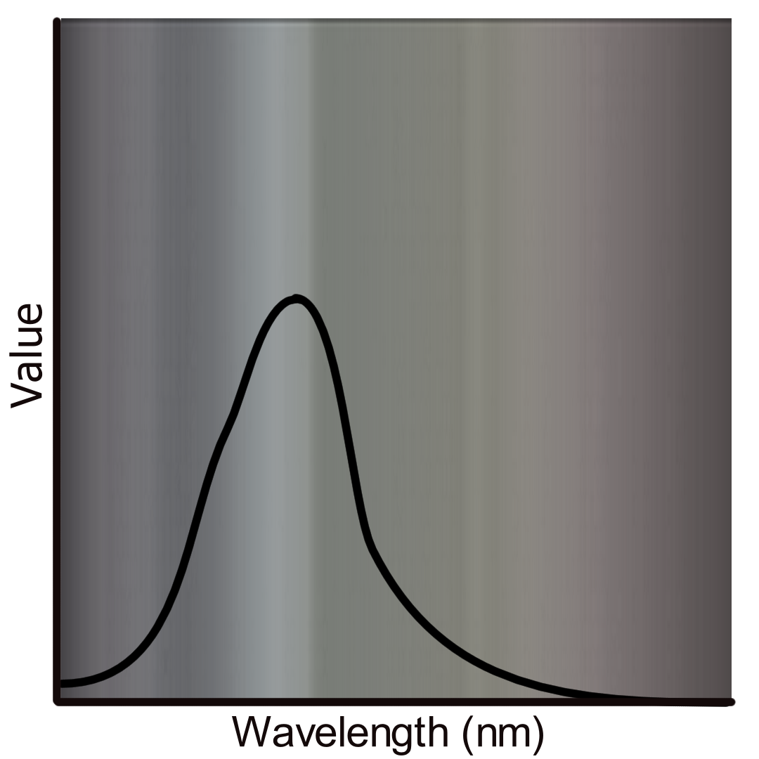
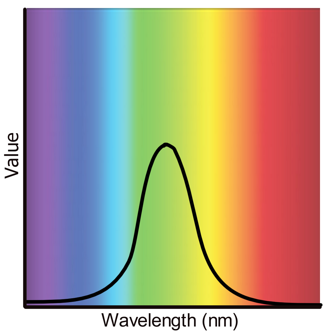
The big difference really is that radiometry includes the entire radiation spectrum and photometry is limited to the visible spectrum and weighted by the responsivity of the human visual system. Radiometry is measured independent of the human visual system, whereas photometry is taking it into account.
Radiometric quantities are great to work with during light transport as they allow for a 1:1 mapping one might find in physics books. For a CG lighter however, it isn’t really a very intuitive measurement. Lighters broadly speaking, aren’t trained physicists with expert training in radiometry. Instead, a lighter’s language tends to be cameras and photography and thus photometric quantities make more sense. Photometric measurements account for the fact that different colours appear as a different brightness for a human observer. For example, since we are more sensitive to green than blue we perceive it as “brighter” than blue. So 2 SPDs, one for a saturated green and one for a saturated blue, even if the SPDs are equivalent for their corresponding colour radiometrically, in terms of photometry we do not perceive blue as bright as we do green. This means we could take a radiometric quantity such as a spectral power distribution and weight it via a luminosity function. Usually for computer graphics the photopic daytime brightness function of the CIE is used. Whilst not exactly the same, I think this is a useful example to bring up. In colorimetric spaces, we have a relative luminance function, which does follow the photometric definition of luminance, but with values normalised to 1 or 100 as the reference white. So for example, if we have an RGB colour and we want to desaturate it, we could simply plus the 3 elements and divide by 3 (calculate the mean). However, this isn’t factoring in the fact we perceive greens brighter than blues for example. So instead of \(Y = (R + G + B) / 3\) we use \(Y = 0.2126R + 0.7152G + 0.0722B\) which weights RGB towards the luminosity function (assuming we are using linear light values). Anyway, by using photometric quantities, this allows us to express radiant power not in Watts, but in lumens which is then called luminous power for instance. For all radiometric quantities, there are equivalent photometric measures. Designing a rendering interface for lighters around this allows an artist to change the colour of a light source and still maintaining the same perceived brightness (which is very important!) in a predictable manner.
It is also important to note that radiometric measurements have equivalent photometric measurements. Here are a few key ones:
| Radiometric Name | Unit | Symbol | Photometric Name | Unit | Symbol |
|---|---|---|---|---|---|
| Radiance | \(W/(m^2 \cdot s_r \cdot m)\) | \(L_\lambda\) | Luminance | \(nit \text{ }\text{ } lm/(m^2 \cdot s_r)\) | \(L_v\) |
| Irradiance | \(W/(m^2 \cdot m)\) | \(E_\lambda\) | Illuminance | \(lux \text{ }\text{ } lm/m^2\) | \(E_v\) |
| Radiosity | \(W/(m^2 \cdot m)\) | \(J_\lambda\) | Luminosity | \(lux \text{ }\text{ } lm/m^2\) | \(J_v\) |
| Radiant Emittance | \(W/(m^2 \cdot m)\) | \(M_\lambda\) | Luminous Exitance | \(lux \text{ }\text{ } lm/m^2\) | \(M_v\) |
| Radiant Intensity | \(W/(m^2 \cdot s_r)\) | \(I_\lambda\) | Luminous Intensity | \(candela \text{ }\text{ } lm/sr\) | \(I_v\) |
| Radiant Power | \(watt \text{ }\text{ } W/m\) | \(\Phi_\lambda\) | Luminous Power | \(lumen \text{ }\text{ } lm\) | \(\Phi_v\) |
| Radiant Energy | \(joule \text{ }\text{ } J/m = W \cdot s/m\) | \(Q_\lambda\) | Luminous Energy | \(talbot \text{ }\text{ } lm \cdot s\) | \(Q_v\) |
Where \(lm\) is lumen, \(W\) is watt, \(sr\) is steradians, \(m\) is metre, \(s\) is second and \(J\) is joule (which can be expressed as watt second).
Path Tracing Methods

From the previous posts, hopefully we have accumulated a good idea of which topics are important in the topic of path tracing. To finish off, now that we’ve covered the very basic foundational knowledge in light transport, we can finish with some techniques for solving light transport.
1) “Simple” Path tracing
Probably this is best described in Kajiya’s paper from 1985. Let’s assume a naive uni-directional path tracer for this example. For constructing paths, this is carried out iteratively by successfully extended the path starting at the camera. This means sampling a pixel, we start from a point on the camera and tracing a ray to the first intersection with the scene. Then, once an intersection is achieved, we check if this is a light source, or not. If it is a light source, we can add up contribution. If not, we randomly generate a new path. We would keep repeating this until we eventually hit a light source. Once that is achieved, we have basically followed (backwards) a potential flight path of a photon in the scene. Remember, at each intersection point we will be evaluating the rendering equation, including any emission, BRDF attenuation, cosine attenuation and other incoming radiance.
2) Next Event Estimation
Naive unidirectional path tracing has a real problem whereby we sample uniformly. This means that even though lights are really important to path tracing, they are not given any sort of additional weight, to help find lights in the scene. Next event estimation tries to solve this. So now, a path can be directly connected to the light source by explicitly sampling the surface area of the area light. While this guarantees finding light sources very efficiently, it does have limitations. This technique disregards the BRDF entirely, which is problematic and in the worst of cases can result in almost no throughput (for near mirror-like specular BRDFs). Ways around this would be to use Multiple Importance sampling whereby light sampling and BRDF sampling is combined for direct illumination.
3) Light tracing
Another technique involves creating a random walk from emissive light sources towards the eye/camera although with this it is very easy to construct symmetric fail cases by putting smooth specular materials between the eye and diffuse surface. However, this technique can be combined via MIS (multiple importance sampling) with previously mentioned techniques to generate more robust estimators. Bidirectional Path Tracing can help render difficult transport paths much more efficiently than with unidirectional path tracing. By using this technique, caustics through glass and highly specular surfaces can be rendered more successfully.
4) Markov Chains
A Markov Chain is a series of points in a state space where the probably of a state appearing at a given position in the sequence depends based on the previous state. Markov Chains are part of the Metropolis Light Transport system. By leveraging the Metropolis algorithm, when light-to-eye paths are successfully found, the algorithm explores nearby paths by modifying the existing path. This can result in difficult light transport paths being solved far, far more quickly than with unidirectional path tracing.
In production, the most popular method of light transport tends to be a uni-directional path tracer, combined with use of multiple importance sampling. This is because it provides a predictable, and relatively simple implementation for engineers and an intuitive interface for artists to use. Bidirectional path tracing can be used for particular instances although overwhelmingly production work is carried out with unidirectional path tracing. More recently, denoising and machine learning techniques are being used to help accelerate light transport. Novel techniques to help build upon the building blocks of Monte Carlo estimation are being developed all the time in the field of path tracing and even more so, now that real-time ray tracing has become increasingly popular.
This was a series of posts that give a basic introduction to some of the topics I felt were most important in path tracing. I hope it has been useful!