Useful Fundamentals for Path Tracing: Part 2
In a nutshell: To calculate the colour of a single pixel, we construct a path from the associated point on our camera sensor towards points in our scene and construct further paths leading to light sources. By calculating how much light is transported from the light to the sensor along this arbitrary path space, we can arrive at an answer for solving the colour of a pixel. In reality, its not possible to compute every single photon present in a scene and all its paths in a scene; it is just too computationally expensive. We instead use Monte Carlo Integration to estimate the real value by firing samples into a scene. With a few samples we can get a rough noisy estimate of the light transport and with more samples we arrive closer to the expected value.
In the previous post we covered some assumptions in computer graphics with regards to light transport. We also had a quick look at photons, scattering events of photons and highlighted the importance of using physically based representations of light across paths in path tracing. With a good understanding of these points, now we can have a look at understanding how much light flows along a constructed transport path.
Constructing Paths and Calculating Transported Light
Here is an illustration of a light transport path:
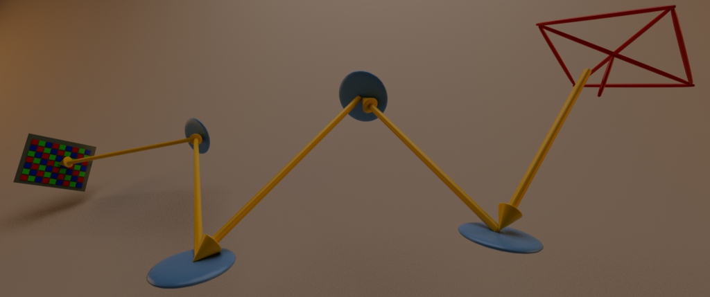
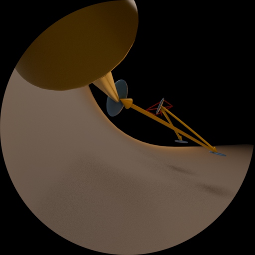
We can represent a light transport path as a list of vertices where each vertex has its own integration domain. Remember, to calculate the light transported to one surface, we perform integration over a unit hemisphere on that point. In rendering where we would be modelling a camera as our measuring device, it would be in the manner of collecting photons per time incident on the pixel area, from given solid angle. Really what this means is that to compute radiant power we need to integrate the measurement contribution from all vertex areas \(dx\) associated with a path. For an example, a path of 5 vertices would need to be integrated over 5 individual surface patches. For rendering an image, we would need to track all possible paths that photons emitted from light sources can take in a scene, including interactions with objects and materials, cosine attenuation, BSDF interaction, sub-surface scattering and volumetric scattering. Finally these photons are accumulated and “counted” on our camera sensor.
The sampling space is typically referred to as the “path space” or \(P\). This would contain a linear list of all possible transport paths, such as \(X =\) {\(x_1, x_2, x_3, x_4, …, x_k\)} \(\in P\). To compute the colour of a pixel (defined as \(I_p\)), we would need to integrate over this space, weighted by a pixel filter \(h_p(X)\) which can also model the camera responsivity. If we generalise light transportation into \(f(X)\), and put this altogether, we can represent a path integral for global illumination:
\[I_p = \int_p h_p(X) \cdot f(X) \text{ } dX\]So this equation basically is telling us that to calculate the colour of a pixel, we integrate the radiant power over the path space (solve the transported light at each path vertex), weighted by a pixel filter.
Using Monte Carlo Estimation
Of course in practise, we are usually not calculating the colour of just one single pixel, with a path length of 5 vertices. We will often be rendering images with millions of pixels often with hundreds of vertex paths associated with each pixel. To solve the integration of these path spaces, many integration methods such as Riemann sums would perform poorly with high dimensional integrals. The industry standard is to use Monte Carlo methods which tends to perform very well with high dimensional integrals. If you are interested, there is a history of using Monte Carlo methods to calculate neutron transport.
Instead of solving an integral analytically, with Monte Carlo methods, we randomly draw samples and evaluate them. The larger the amount of samples \(N\), the closer we converge to the expected value. These randomly drawn samples are from a probability distribution functions (PDFs). I will cover PDFs in more detail in a future post but for now all we need to be aware of is that to draw a sample from a PDF, we generate a uniform number in range \([0, 1]\) and feed that into a PDF. This then returns a randomly generated number. As long as a PDF integrates to 1, we can have any distribution, even a distribution that tends to generate more samples in one area, and less samples in another (which is desirable in importance sampling).
In probability theory, the expected value of \(x\), would be defined as:
\[E (x) = \int x \cdot p(x) \text{ } dx\]Where to solve the integral, we draw random samples from \(x\). And a Monte Carlo estimator with \(N\) samples would look like:
\[\frac{1}N \sum_{i=1}^N x \approx E (x)\]So applying this to the global illumination integral from above we would get:
\[\frac{1}N \sum_{i=1}^N \frac{h_p(x) \cdot f(x)} {p(x)} \approx I_p\]Note that in order to match the definition of the expected value, we need to divide by the PDF, \(p(x)\).
The PDF is basically drawing random samples along any distribution function, which we can choose. For example it could just be a flat value \(\frac{1}{2\pi}\) for all inputs. In theory any PDF would eventually converge to the expected value, but our goal in rendering is to arrive at approximately the correct answer with as few samples as possible (faster convergence). This means we will want to use a PDF that looks similar to function \(f(x)\). This is easier said than done, though there are ways we can approach this. The key one is using importance sampling where we draw more samples in areas of the integral that are likely to contribute more to the final answer. In the future I will do a post dedicated to importance sampling but for now, lets just be aware that it exists and it is a method to arrive at a less noisy answer with fewer samples \(N\).
To illustrate how Monte Carlo estimation works in the context of integration, here’s an example of a curve which we can solve analytically and with Monte Carlo
\[y = x^2 + 1\]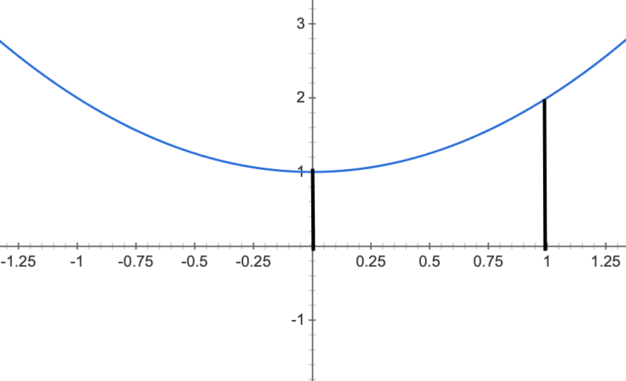
Lets say the area under this curve, bounded by x = 0 and x = 1 represents the incident radiance at a point on our camera sensor, \(L_i\). To solve analytically we would do the following steps:
\[Area = \int_0^1 (x^2 + 1) \text{ }dx\] \[= \Big[ \frac{x^3}3 + x \Big]_0^1\] \[= \Big[ \frac{1}3 + 1 \Big] - \Big[ 0\Big]\]Which gives us an exact solution of \(\frac{4} 3\) or as a decimal \(1.333\) recurring. Now, instead of a fairly simple quadratic equation, if we pretend this was a highly complex, recursive equation that we were unable to solve analytically (which is the case in the rendering equation). We can instead use samples along the domain of \([0, 1]\) and average the results, in the hope it gives us a somewhat correct answer.
Let’s try this with some code.
int main()
{
    int samples = 8;
    float area = 0.0f;
    UniformSampler *sampler;

    for (int i = 0; i < samples; ++i)
    {
        float random_sample = sampler->generate();
        area +=(powf(random_sample, 2.0f) + 1.0f);  // y = x^2 + 1
    }
    area /= float(samples); // Average result
    std::cout<<"Using "<<samples<<" samples. Estimated area is "<<area<<"\n";

    return EXIT_SUCCESS;
}
Okay, so now if we test this with 2 samples we get:
> Using 2 samples. Estimated area is 1.4318That’s unfortunately not very close! What if we a different range of samples?
> Using 8 samples. Estimated area is 1.29646> Using 64 samples. Estimated area is 1.30208> Using 2048 samples. Estimated area is 1.33141Eventually, we converge to an answer that’s pretty close to what we solved analytically. We would expect the variance to decrease the more samples we use. In the absence of an exact solution, Monte Carlo estimation performs well for path tracing. Instead of solving the light transport for all possible photons in a scene, we instead estimate the light transport with many samples of potential paths. The numerical error of low samples in rendering will manifest in image noise:
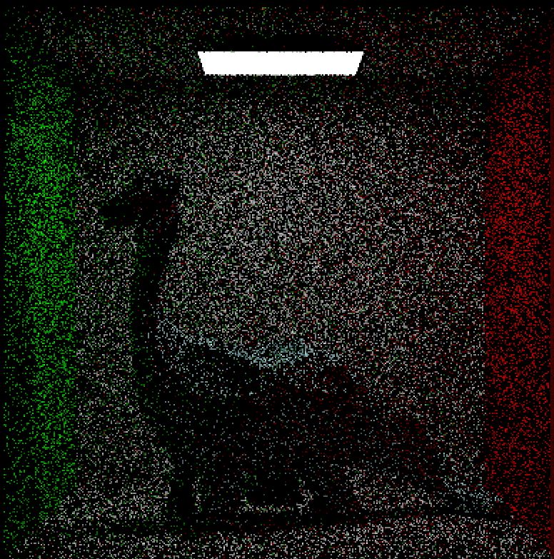
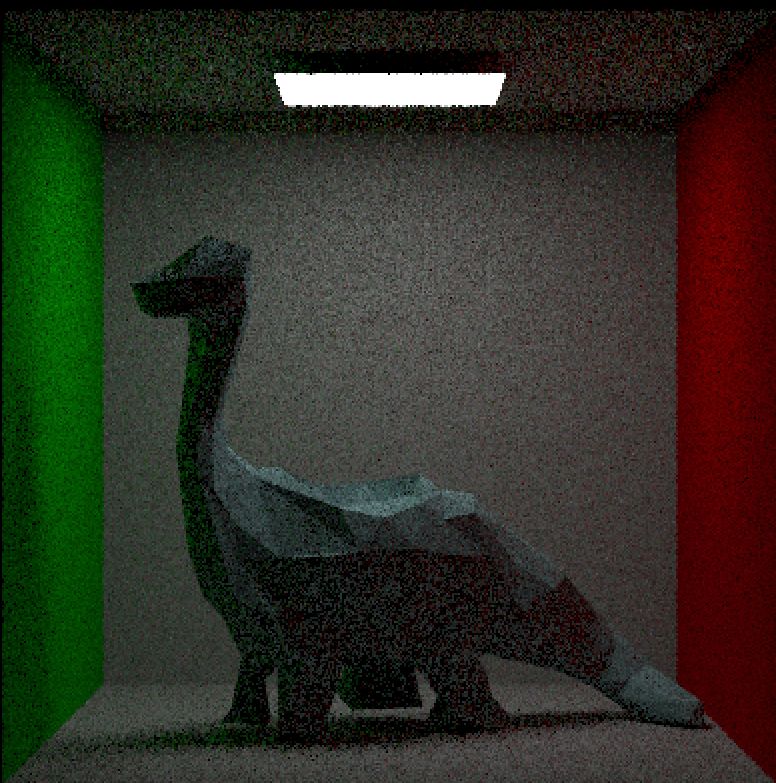
So to summarise, we are sending out random samples, averaging them and slowly converging to a correct answer, with more samples (N). This is exactly the method we use to solve the light transport in path tracing.
That’s it for this post! At this point we should understand that path tracing uses light transport, measuring areas, solid angles, time intervals and photon scattering. To calculate how much light is transported, we construct paths from the camera sensor to light sources and evaluate integrals on each vertex. Since this often leads to high dimensional integrals, we instead use Monte Carlo Integration to estimate the correct answer, with samples drawn from a PDF. In the next post, we will take a look at how we actually form colour in rendering!