Useful Fundamentals for Path Tracing: Part 1
In a nutshell: Path tracing involves constructing lines/paths of intersection towards light sources (both directly and indirectly). Light is transported along this constructed path space. We can use the radiative transfer equation and understanding how to measure photons as the physical basis of this.
This will be the first in a short series of blog posts where I cover some of the fundamentals for path tracing and light transport. This will by no means be comprehensive. Instead, I’ll write starting points for topics I think are important for path tracing.
With Animation and Visual Effects studios fully transitioned to path tracing, and with game engines embracing real-time ray tracing, this is a really exciting time to be involved with light transport! The target audience for these blog posts are people who are curious to know more, but are a bit intimidated by all the technical literature out there, much like I was back when I was starting out. For that reason I won’t rely too much on equations and instead just try make the broad concepts more understandable.
Lets start with the basics. Say we are wanting to create a rendering solution such that we give a program an input scene and get an output image. What would the input scene consist of? We would most likely have geometry (represented by triangle meshes, subdivision surfaces etc), we would have lights (area lights, distant lights, dome lights), texture maps, material descriptions (both procedurally generated and artist generated) and finally a camera (with input properties such as lens type, sensor width etc). Using these inputs we can create highly complex and realistic images by simulating the light transport to be physically plausible. So, now let us have a look at how we could try quantify light transport.

To find a way of quantifying light transport into some tangible measurement, we need to derive some standardised measurement function. This is important; if we arbitrarily create measuring methods without some scientific foundation, we have no foundation in reality! If the goal is photorealistic light transport, then of course we need to have path tracing based in some sort of reality. In essence, we are answering the question of “what colour is this pixel?” with a solution informed by application of optical physics and the radiative transfer equation. So this means along our ray paths, we need to measure some real-world measurement of a physical quantity. By the way, when we refer to a ray, this is essentially an infinitesimally small line of direction (\(\boldsymbol d\)) originating from an infinitesimally small position (\(o\)). The most common representation that we will see in computer graphics is \(r(t) = o + t\boldsymbol d\). This is a parametric equation where the parameter \(t\) is the length along this ray. We will revisit this later. For now, lets begin with some common assumptions in the field of computer graphics.
Assumptions
- We will only be concerned with elastic scattering. So basically this means we are assuming there is no energy transfer between wavelengths (meaning no photoluminescence) We will assume that we will only really be concerned with ray optics (or geometric optics) and not worry about wave optics, electromagnetic optics or quantum optics.
- Photons are travelling along straight lines, this means assuming the index of refraction does not vary continuously but only at intersected points (perhaps a material description has an IOR of 1.47), so unless otherwise specified we assume an IOR of 1.0 (for air).
- We also assume light is not affected by gravity as it would be on astronomical scales (and generally most scenes involve an indoor environment or outdoor landscapes)
- Light consists of particles (photons) and not waves, for the purposes of measuring radiance
Some Notes on Photons
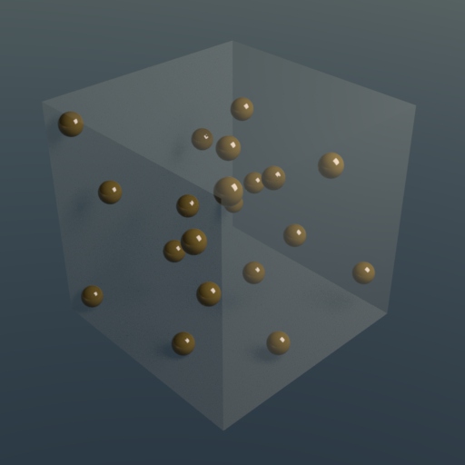
Since we can assume light consists of particles (photons), we can move towards our goal of simulating transport by starting with a simple exercise of counting photons in a given volume over a given time interval. A photon is a type of elementary particle and is critical in understanding the field of electromagnetic radiation. Visible light (which is what we are trying to simulate) is part of the electromagnetic spectrum, between 380-780 nanometers. We should be aware that a singular photon corresponds to an atomic portion of energy \(E\) measured in joules \(J\). To reach our goal of physical light transport, it could begin with the idea of “counting” or “accumulating” photons on a sensor. To measure a single photon, we would use the equation below. Remember that a single photon corresponds to an atomic portion of energy \(E\) measured in joules \(J\).
\[E = \frac{h \cdot c_m} {\lambda} \text{ } [J].\]With \(h\) \(\approx\) \(6.62607004 \cdot 10^{-34} [m^2kg/s = Js]\) being Planck’s constant and \(c_m = \frac{c} {\eta_m}\) is the speed of light in a material with an index of refraction \(\eta_m\). This is slightly slower than the speed of light in a vacuum, which also has a fixed constant \(c = 299792458 \text{ } m/s\). \(\lambda\) is the wavelength of the photon. The wavelength is measured in nanometers and we can determine where the photon lies on the electromagnetic spectrum based on this. For our purposes though, we will only be using the wavelength to calculate colour, so really we only care about wavelengths in the domain of visible light.
Now, to determine the overall radiant energy in a certain volume all we need to do is count the photons and calculate the sum of their energies. For example, if they all had the exact same wavelength, we know they’d have the same energies so we can multiply the energy by the number of photons in a volume. This gives us our answer.
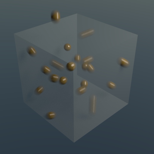
Hopefully this helps demonstrate how modelling photons could be useful. Unfortunately in reality, photons are not stationary and move very quickly. So, rather than counting the photons a more practically useful quantity is to measure how many photons pass through a certain volume per time. This is referred to as Radiant Power or Flux.
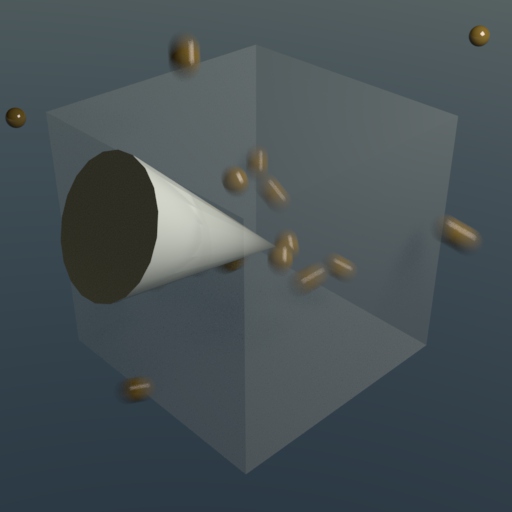
To consider the direction of a photon, we need a measure of directions. A 2D measure space we can use is the solid angle, this is defined as the area of a piece of surface projected onto a unit sphere. To quickly explain a projected solid angle, if you imagine a unit sphere (or hemisphere) on the ground, projecting the sun and moon would roughly create the same solid angle. Even though the sun is many, many times larger than the moon, it is many many times further away from earth than the moon. Thus, they have similar solid angles.
To measure the area (i.e. to integrate) in this domain, we typically would re-parameterise the domain from cartesian direction vectors \((x, y, z)\) into spherical coordinates \((\theta, \phi)\), e.g. using latitude and longitude to make it more intuitive.
We consider photons to live in “phase space”, where they have a 3D \((x, y, z)\) position and a 2D direction \((\theta, \phi)\), which we can parametrise as \((x, \omega) \text{ } \varepsilon \text{ } V \times \Omega\). Now, we should have an idea of how to count photons, per time, per volume and per solid angle. Ideally we would count some placeholder quantity with some imaginary measurement device that only counts photons inside a certain 3D volume if their direction falls within the solid angle subtended by a certain imaginary funnel.
Photon Scattering Events
As we have seen above, photons will move in and out of an observed volume over time, but they also have scattering events. Lets quickly cover what ways a photon can be changed via a scattering event. The most basic is photon emission, where particles emit light (a light source, maybe a blackbody emitter). There are 2 other things that clearly change photon count in a certain observed volume in phase space (remember, a space where photons have 3D positions and 2D directions they are moving along). The most natural is streaming, which is a photon entering or leaving a volume by just continuing along its set path, without interacting with matter inside our observed volume. The second event that clearly changes photon count is collision, where the photon interacts with matter inside of the observed volume. In the event of collision, the photon may be scattered or absorbed. While absorption is always results in a loss of photons (transferred into heat energy, which we do not model for light transport), scattering may mean both: the new direction of the photon could be inside the currently considered solid angle of the phase space, or it might have left it entirely. Let’s define these terms a bit further.
Absorption. Collisions with an absorbing particle is easy to model since for our purposes in path tracing, all that happens is a photon disappears. All we need to model is how often such an event might happen. Typically, a statistical model is what is used to determine this. If you are familiar with microfacet BRDFs, then its sort of a similar idea, where we use a function to statistically model a series of microfacet normals.
Emission is very similar to absorption in that a blackbody emitter model dictates every photon intersecting an emitting particle is absorbed, rather than reflected. This means emission comes with a loss term, very similar to the one that would be found in absorption.
Streaming. To calculate how many photons enter and leave the current piece of phase space, \(V \times \Omega\) we want to count the number of photons passing through the spatial boundaries of \(V\), which is written as \(\partial V\).
Scattering. Once a photon collides with a particle it can also be scattered (experience a change of direction \(\omega\)). Since we are limiting ourselves to elastic scattering, the energy of the photon remains unchanged during the scattering event. This means the wavelength especially stays the same, limiting our analysis to one wavelength at a time, and thus solving the path tracing one wavelength at a time. Depending on the new direction of the scattering, this may result in a gain or loss. The photon might get scattered into the observed solid angle of our piece of phase space, or leave it.
So the key scattering events here are absorption, emission and scattering for energy transfer. Because we are considering all the possible ways a photon can be added or lost, doing so would mean when solving this, we would get zero (all scattering events have been considered). Using these events we arrive at the concept of radiative transfer. Radiative transfer is the physical phenomena of energy transfer by electromagnetic radiation. Rather than go into detail on the derivation of the radiative transfer equation I’ll instead just present the 2 more commonly used equations in path tracing, and this will highlight how these photon scattering events translate into a path tracing equation.
\[L_o(x, \omega_o) = L_e + \int_\Omega f_r(x, \omega_i, \omega_o)L_i(x, \omega_i)(\omega_i \cdot n) d\omega_i\]This is a version of the recursive path tracing equation by Kajiya. We can see that the light arriving at point \(x\) is calculated by adding any emission from \(x\) directly, and then the sum of 3 factors across a unit hemisphere \(\Omega\). The first \(f_r\) is the BSDF (bidirectional scattering distribution function) which describes the material at point \(x\) (The texture colour, glossiness etc), the second term is the amount of light arriving to \(x\) from another point and finally the third term is the cosine attenuation factor.
\[L = L_e + \boldsymbol T L\]Is simplified equation from Eric Veach using a linear transport operator \(\boldsymbol T\) where it says the light at a given point is equal to light emitted by that point, plus any light that is transported to the point (either indirectly or directly from lights).
That brings us to the end of this post! This is very much just scratching the surface on these topics, but hopefully it is clear that physically based path tracing is very much based in real-world physics. Even though path tracing involes a lot of ray-object intersections and tracing rays in a scene, its important to note that the thing we are transporting along these paths (light) needs to be measured and handled in a physically based manner. This is why I personally think its good to be aware of what radiative transfer is, methods of measuring photons and understanding that we use integrals and solid angles to measure the transport of light energy along paths. In the next blog post I’ll introduce how we use Monte Carlo integration to solve the rendering equation.